\(H_0^B\): do the class proportions shift with diagnostic era and age at diagnosis?#

Definition

\(H_0^B\) (prevalence). Null: the four class prevalences are constant across diagnostic era and across age at diagnosis; each class holds the same share of the diagnosed population at every point on an axis. Alternative: at least one proportion trends along an axis, for example the developmental class shrinking toward later diagnosis. Estimand: the mixing proportion \(\pi_k\) of autism class \(k\) read as a function of the axis, \(\pi_k(\text{axis})\). This is a question about size, distinct from the profile-shape questions the invariance reads answer, and it is reported on its own.

Status

The null is rejected on both axes: every class proportion trends. Along age at diagnosis the shift is stark. Mixed ASD with developmental delay falls from about \(0.35\) of the earliest-diagnosed to under \(0.01\) of the latest (per-year log-odds slope \(-0.35\), odds ratio \(0.71\)), while Social or behavioral rises from about \(0.24\) to about \(0.60\) (slope \(+0.13\)). Along diagnostic era the same pair leads more gently: the developmental class falls from about \(0.26\) to about \(0.09\) across the era span (slope \(-0.08\)) as the social class grows. The joint likelihood-ratio test of class on the axis against a constant saturates at the full sample (\(\chi^2 = 365\) on \(3\) degrees of freedom for era, \(\chi^2 = 1204\) for age), so the read is the size and shape of each class’s trend, not the binary reject. The corrected and naive estimates agree to three or four decimal places, so the reference posteriors are confident and the naive cross-check corroborates. The age trends survive adjustment for measurement timing and sex; on era the Social or behavioral rise is nullified by that adjustment while the developmental decline and the Broadly affected rise persist.

Method#

Prevalence is a different quantity from profile shape, and the two can move independently: a class can hold its shape while its size moves, or move its shape while its size holds. Holding the classes fixed separates the two. With the profiles fixed at the measurement-only reference fit, a trend in the mixing proportion is prevalence drift alone, uncontaminated by any change in profile shape.

The frozen reference gives every proband a posterior over the four classes, and the stage regresses class membership on the axis using those responsibilities. The direct approach regresses each proband’s hard (modal) class label on the axis. It is transparent but biased: the hard label is a noisy reading of the true latent class, because the posterior is not a point mass, so a share of the labels are wrong, and regressing a mislabelled outcome on the axis pulls a real slope toward zero and can invent one where there is none. This is the classify-analyse bias of three-step estimator latent-class analysis.

The primary read corrects it. The modal assignment is treated as a single categorical measurement of the true class whose error probabilities are fixed at the confusion matrix of the frozen posteriors, and the structural model, a multinomial logistic regression of the true class on the axis, is fitted by expectation-maximization with that measurement model held fixed. The correction removes the attenuation without touching the mixture. A naive multinomial logit on the hard labels runs beside it as an uncorrected cross-check. Uncertainty is a family-clustered bootstrap resampling SPARK families, the same convention the effect-size reads use: each replicate recomputes the confusion matrix and the corrected fit, so every slope and the proportion curve carry a percentile interval, a confidence band, and each slope a two-sided bootstrap \(p\)-value. Significance is false discovery rate-controlled across the four classes at \(q = 0.05\), separately for each estimator.

This is the analysis prevalence stage. The correction mechanics, and the correctness gates that check it (including that it de-attenuates a known slope where the naive one does not), are in the guide on measuring prevalence drift.

Experimental design decisions#

Frozen classes. The invariance question is about profile shape; prevalence is about size, and the two come apart only if the classes are held fixed. The stage regresses on the axis with the reference posteriors.
Bias-corrected read leads, naive read corroborates. The classify-analyse attenuation is corrected as a guarantee, so the result stands without assuming the posteriors are error-free; the naive hard-label logit runs beside it as a transparent cross-check.
Families resampled, not probands. Siblings share a family and correlate, so resampling whole families gives an honest, wider interval.
An adjusted sensitivity. The corrected axis slope is estimated net of sex, the measurement-to-diagnosis lag, and age at evaluation, so a trend that survives is more than a measurement-timing or sex-composition artefact.

Results#

The runs are on SPARK 2026-03-23 (\(11{,}704\) probands) against the measurement-only reference fit 41ab0e38 at \(500\) bootstrap replicates: the era run has a diagnosis year for \(98.3\) per cent of probands and the age run an age at diagnosis for \(98.4\) per cent. The pooled proportions, the classes’ shares over the whole cohort, are \(0.39\) for Social or behavioral, \(0.25\) for Moderate challenges, \(0.21\) for Broadly affected, and \(0.16\) for Mixed ASD with developmental delay.

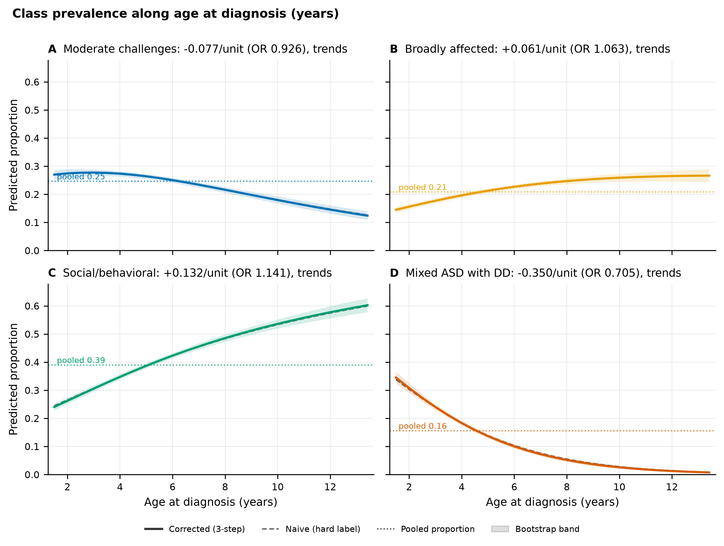
Predicted proportion of each class as a function of age at diagnosis, one panel per class, with bootstrap bands — Class prevalence along age at diagnosis, one panel per class: the solid line is the corrected proportion curve, the shaded band its family-clustered bootstrap interval, the thin dashed line the naive hard-label cross-check, and the dotted horizontal line the pooled proportion the class trends away from. How to read it: a curve above its dotted pooled line is a class over-represented at that age and an upward slope a class growing, so the developmental band falling to almost nothing while the social base rises is the composition shifting from developmental to social presentations as diagnosis moves later in life. Rendered by `figures.prevalence` (`figures prevalence --axis age_at_diagnosis`).#

Across age at diagnosis all four classes trend, and the developmental split is the headline. Mixed ASD with developmental delay falls from about \(0.35\) among those diagnosed near age two to under \(0.01\) among those diagnosed in the early teens, while Social or behavioral runs the other way from about \(0.24\) to about \(0.60\); Broadly affected rises gently and Moderate challenges declines. This is the expected shape of a diagnosed population, the developmental class recognised early and thinning among the late-diagnosed where the social presentations take over.

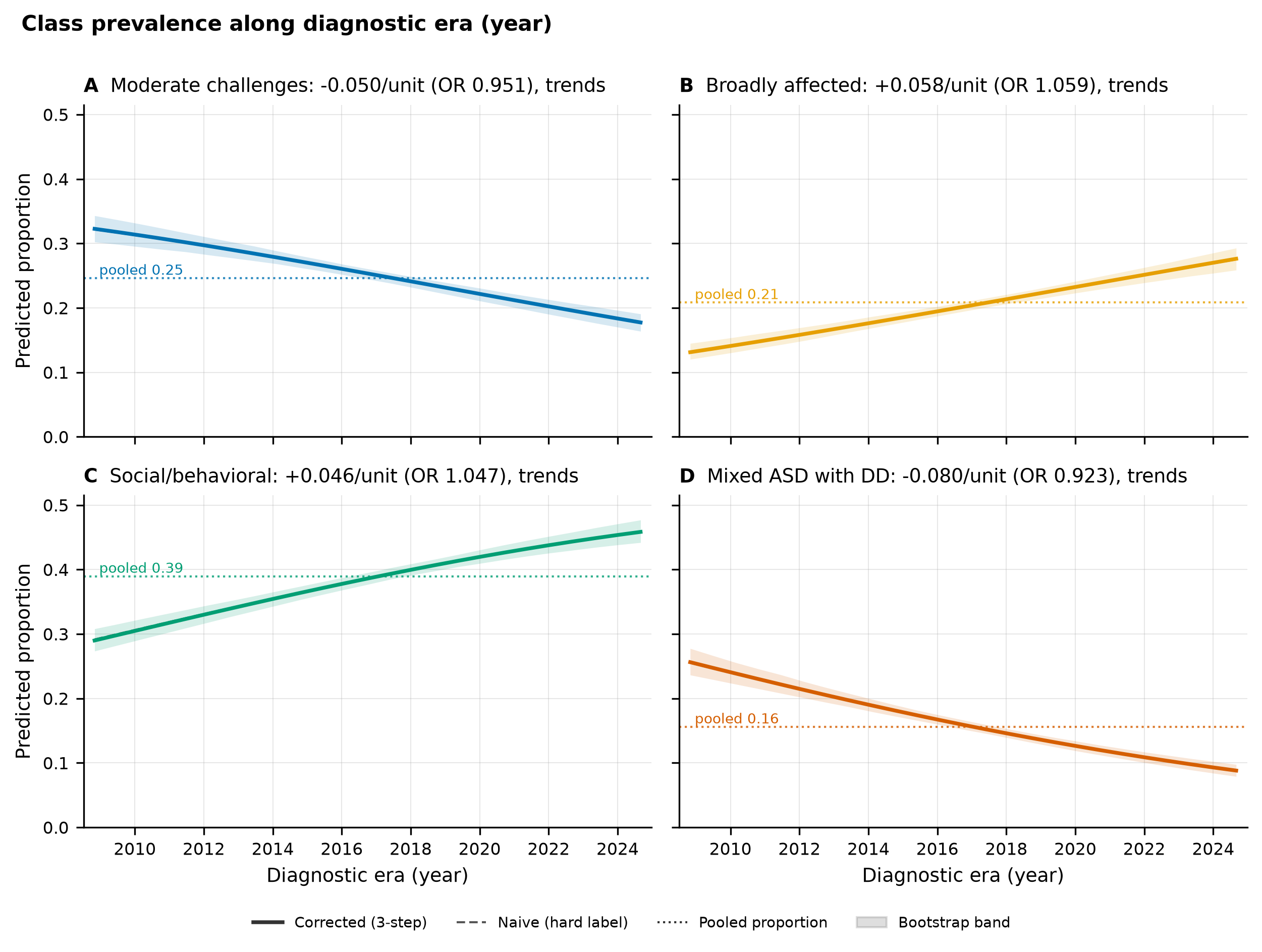
Predicted proportion of each class as a function of diagnostic era, one panel per class, with bootstrap bands — The same read along diagnostic era, a milder version of the same shift. How to read it: as above, with diagnosis year on the horizontal axis. The developmental class falls from about \(0.26\) among the earliest-diagnosed years to about \(0.09\) in the recent years while the social class grows, and Broadly affected and Moderate challenges shift by smaller amounts. Rendered by `figures.prevalence` (`figures prevalence --axis era`).#

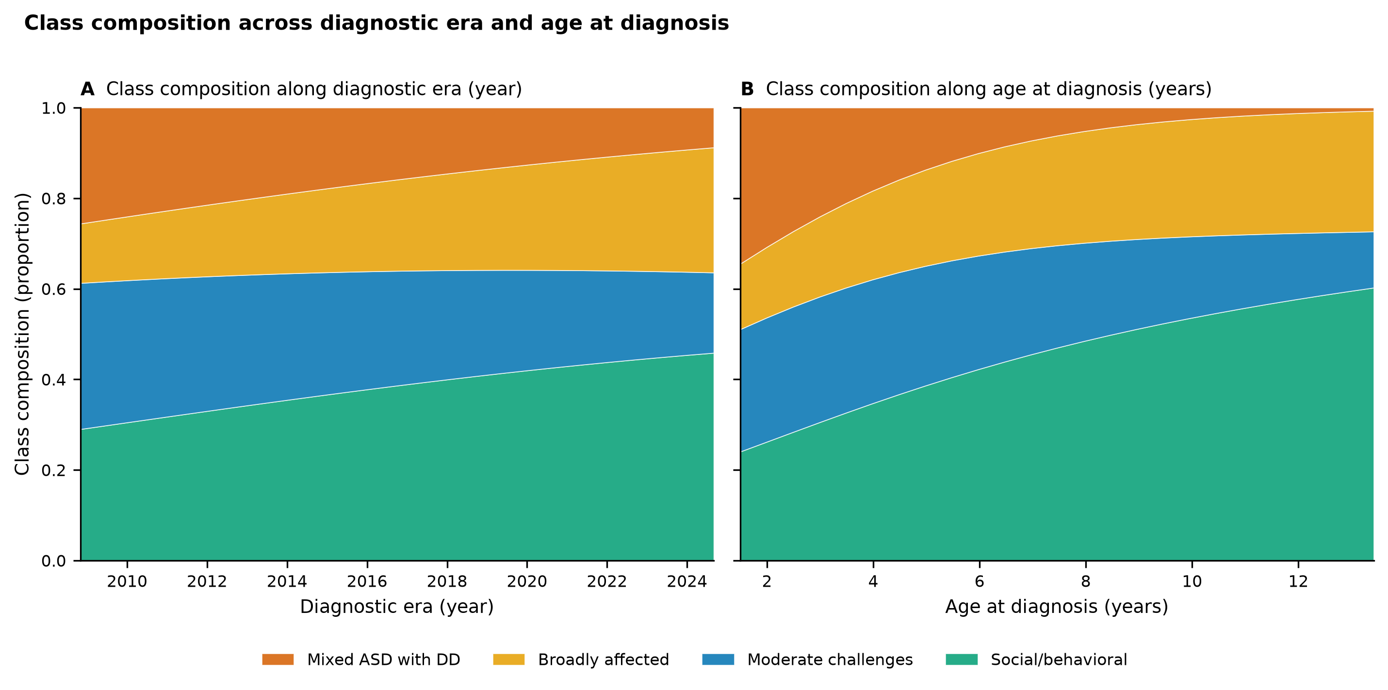
The four class proportions stacked to one across diagnostic era (left) and age at diagnosis (right) — Both results as a composition, the four corrected proportions summing to one at every point: diagnostic era on the left and age at diagnosis on the right, sharing the vertical scale so the two trades compare directly. How to read it: because the proportions are stacked to one each panel reads as a single shifting mixture, the Social or behavioral base growing as the developmental band at the top thins to almost nothing. Panel B is the starker version, the developmental band all but vanishing among the late-diagnosed, and panel A the gentler era echo of the same trade. Rendered by `figures.prevalence` (`figures prevalence --layout stacked-pair`).#

Diagnostic era carries a secondary read, a pre and post-2013 contrast that marks the DSM-5 boundary. Every class shifts across it in the same sense as its continuous trend and by a larger step: the odds of the Broadly affected class are about \(1.6\) times higher after 2013 and of the Social or behavioral class about \(1.5\) times, while the odds of the Moderate challenges and Mixed ASD with developmental delay classes are about \(0.68\) and \(0.58\) times their pre-2013 values. The boundary is a descriptor overlaid on a continuous trend, not a claim that the change happens at the boundary.

A prevalence trend across era could reflect a change in who is diagnosed or an artefact of when they were measured relative to diagnosis, so the adjusted read fits the corrected axis slope net of sex, the measurement-to-diagnosis lag, and age at evaluation. On age at diagnosis every class keeps its trend, the developmental decline and the social rise included, so the age composition shift is more than a measurement-timing effect. On era the picture divides: the Broadly affected rise and the Mixed ASD with developmental delay decline survive, but the Social or behavioral era rise is nullified, its adjusted slope near zero with an interval covering it. So the growing share of the social class across recent years tracks measurement timing rather than a change in the diagnosed population.

Handling the null#

The decision is a per-class trend read, not a reject-or-not on the joint \(p\)-value. At the full sample the joint likelihood-ratio test of class on the axis against a constant saturates (\(\chi^2 = 365\) on \(3\) degrees of freedom for era, \(\chi^2 = 1204\) for age), so a constant-proportion null is rejected outright and the interpretation rests on each class’s slope, its sign, its size, and its bootstrap interval. On both axes all four per-class slopes trend, with the developmental decline and the social rise the largest and clearest, so \(H_0^B\) is rejected on both. The adjusted read qualifies one strand of the era verdict rather than overturning it: the Social or behavioral era rise is a measurement-timing signal, while the developmental decline and the Broadly affected rise, and the whole age-axis result, survive adjustment.

Discussion#

The class proportions are not constant. The diagnosed autism population shifts from developmental toward social presentations as diagnosis moves later in life and, more mildly, into more recent years, and on the age axis that shift is not an artefact of when the measurements were taken. The read is conditional on the pooled fit: it freezes the reference posteriors and regresses on the axis, so it measures how the fixed classes’ sizes shift. Holding the profiles fixed is what lets a size change be read as prevalence drift alone, separate from any change in profile shape.