\(H_0^A\) and \(H_0^D\): are the class profiles invariant, and is any drift small?#

Definition

\(H_0^A\) (invariance). Null: the four class profiles are invariant to diagnostic era and to age at diagnosis; the class-conditional measurement parameters do not vary with the axis. Alternative: at least one class-conditional parameter varies systematically with the axis. Estimand: the class-parameter-by-axis association, read per class as the separation-scaled displacement of the local class centroid along the axis.

\(H_0^D\) (magnitude). Null: any detected drift lies within finite-sample estimation error and is negligible against the between-class separation. Alternative: the drift is both distinguishable from sampling noise and non-trivial relative to the gap between classes. Estimand: the separation-scaled displacement as an absolute size, with a capture fraction that flags drift lying outside the between-class discriminant plane.

Status

Both nulls are rejected on both axes. In between-class separation units (one unit is the mean inter-class gap), the endpoint displacement averages about \(0.18\) of a class gap along diagnosis year and about \(0.39\) along age at diagnosis, largest for the developmental class (Mixed ASD with developmental delay, \(0.30\) era and \(0.70\) age). The control panel sits at about \(0.21\) (household income), \(0.14\) (area deprivation), and \(0.09\) (a random ordering). Age at diagnosis clears every control for all four classes; diagnostic era splits, with Moderate challenges and Mixed ASD with developmental delay clearing the covariate controls while Broadly affected and Social or behavioral clear only the random floor. The paired specificity bootstrap rejects at its floor (\(p = 0.0005\)) on both axes. The drift is not small either (\(H_0^D\) rejected), and the capture fractions are small, so most of the movement is high-dimensional and out of the plane the trajectory figures draw.

Method#

Measurement invariance is an exact point null: no real class profile sits exactly on it, so at the reference sample size (about \(11{,}700\) probands) a test of exact invariance always rejects. The primary read therefore recasts both nulls as a null-free effect size, the size of a class’s profile drift measured against the gap between classes, and demotes the saturated significance test to corroboration.

Hold the four classes as Litman et al. defined them and freeze the reference responsibilities (the model’s predict_proba). For a focal point \(f\) on the axis, weight each proband by a Gaussian kernel around \(f\) and read the responsibility-weighted local centroid of class \(k\),

\[ \mu_k(f) = \frac{\sum_i w_i(f)\,r_{ik}\,x_i}{\sum_i w_i(f)\,r_{ik}}, \]

the local structural equation modelling estimator, with the bandwidth set so each focal fit carries about \(1{,}000\) effective probands. The per-feature displacement \(d_k(f) = \mu_k(f) - \mu_k\) is kept full-dimensional; a magnitude is its standardised Euclidean norm over a group of features, divided by the between-class separation. The norm sums the per-feature displacements rather than averaging them, so this separation-unit magnitude is a comparative scale that grows with the number of features summed over; dividing it by the square root of that count reads it back as an absolute fraction of a class gap (about a fifth on diagnosis year). Uncertainty is a family-clustered bootstrap: families are resampled with replacement (SPARK groups siblings into families, so they move together) and the local centroids recomputed, giving a per-point confidence band. Per-feature tests are false discovery rate-controlled across the four classes and the features at \(q = 0.05\).

The class trajectories are drawn in the fixed linear discriminant analysis plane, which is two-dimensional while the displacement is not, so each class carries a capture fraction, the share of its displacement lying in the plane. A low capture means the picture understates the movement; the full-dimensional magnitude is the authoritative number.

This is the analysis invariance-trajectory stage; the separation and the distances it is read against are the class-drift machinery.

Experimental design decisions#

Measurement-only reference. The invariance question is about the measurement parameters, so the read runs on the marginal fit (analysis fit --no-covariates), not the covariate model.
Per-class specificity, not the between-class mean. A mean over classes hides drift concentrated in one class, so a class is judged specific on its own displacement against its own controls.
A random-order floor, no orthogonality assumption. The confirmatory control is the random ordering, the one baseline guaranteed to carry no structure; any covariate control would assume the covariate is orthogonal to timing, which the data cannot guarantee. The displacement atlas reports the timing axes against every other continuous or ordered non-modelling variable, with the covariates as context and the random order as the floor. The 238 clustered features and held-out phenotype instruments are excluded, the former as circular, the latter as a non-null phenotype ceiling (choosing the specificity controls).
Families resampled, not probands. Siblings share a family and correlate, so resampling whole families gives an honest, wider band.

Results#

The two timing axes tell a consistent story with an honest split. Age at diagnosis clears the random floor for all four classes and is the larger effect, carried by the developmental class (Mixed ASD with developmental delay moves furthest, endpoint about \(0.70\) separation units, roughly seven tenths of a class gap). Diagnosis year clears the random floor too, on the mean and per class, though its displacement sits among the covariate axes rather than above them. Roughly a third of the per-feature displacements survive the false-discovery step for diagnosis year and over half for age at diagnosis, so the drift is pervasive but not total: most single features stay within sampling noise while the profiles as a whole move.

The displacement atlas places the two timing axes among every other continuous or ordered non-modelling variable, so the timing effect is read against a whole panel of orderings rather than a hand-picked few. The panel now spans the demographic orderings too (parental education, the family-history counts, inferred parental age at birth, the perinatal-complication count), and none of them rivals the timing axes.

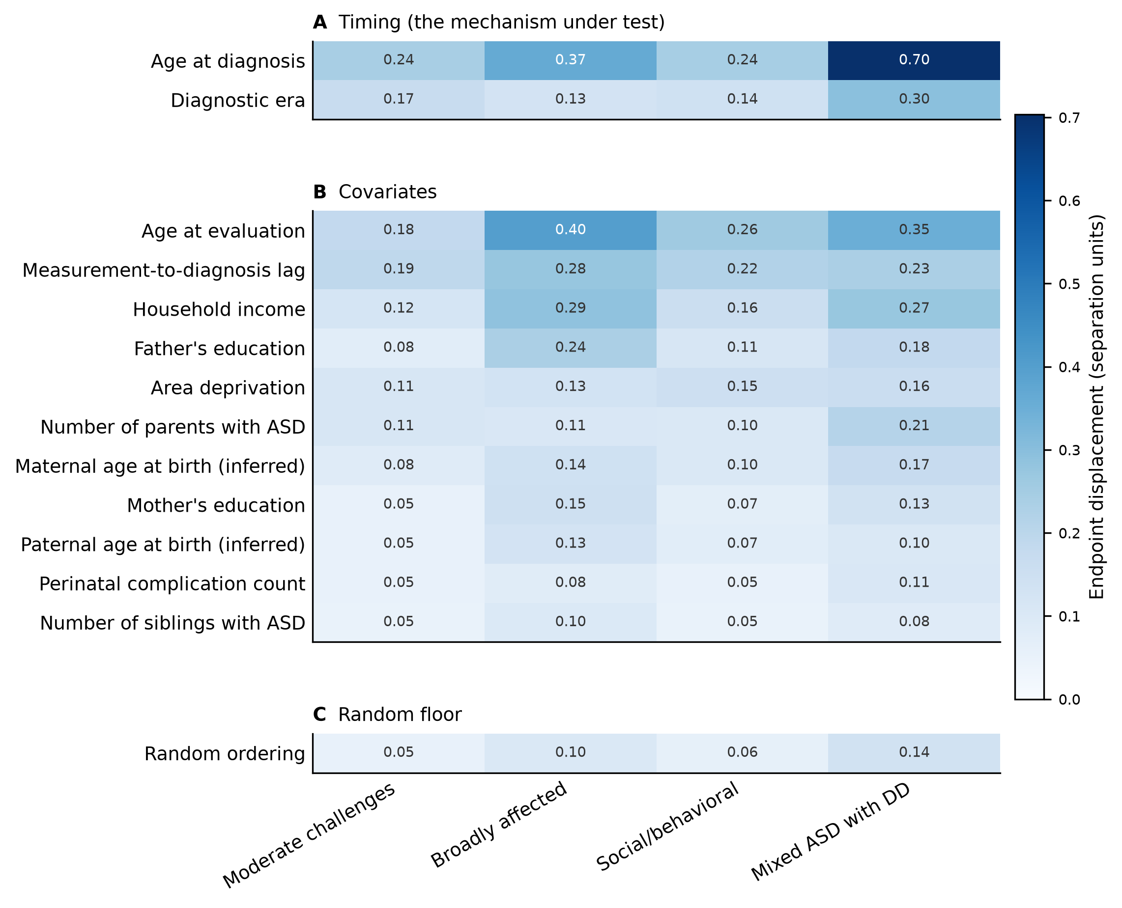
Per-class endpoint displacement along every non-modelling ordering axis, grouped by kind — Per-class endpoint displacement (separation units, the mean inter-class gap) along every non-modelling ordering axis, grouped into panels by kind: the timing axes (A), the covariate pool (B), and the random-order floor (C). Panel B spans the demographic orderings as well as the two chosen covariate controls: household income and area deprivation, parental education, the family-history counts, inferred parental age at birth, and the perinatal-complication count. Within each panel the rows run from the largest class-summed mover to the smallest. Age at diagnosis moves the classes most, led by the developmental class. Most axes clear the random floor, but the weakest demographic orderings (sibling ASD count, the perinatal-complication count) sit at or below it, so they carry no drift beyond sampling noise. The 238 clustered features and held-out phenotype instruments are excluded as circular or as a non-null phenotype ceiling. Rendered by `figures.atlas` (`figures atlas`).#

The capture fractions are all small, near what a random direction would give, so the drift is high-dimensional and mostly out of the between-class discriminant plane. In root-mean-square terms the diagnosis-year magnitude is about a fifth of a class gap.

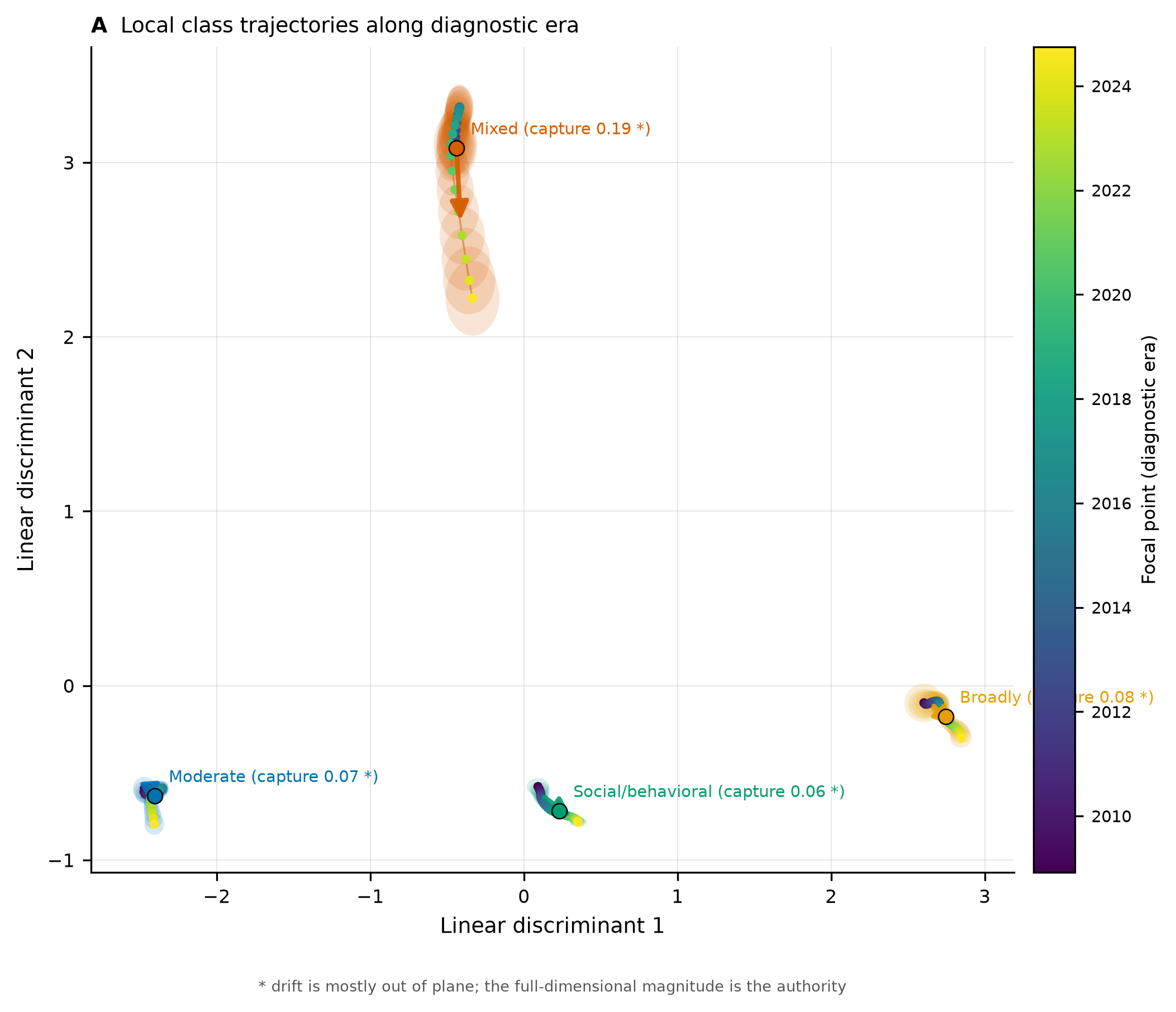
Four class centroids in the discriminant plane, each with a short local trajectory along diagnosis year — Local class trajectories along diagnosis year in the discriminant plane, coloured earliest to latest with the bootstrap band as pale ellipses. How to read it: the four anchors sit far apart, and each class traces a short path. Every class is flagged, its capture fraction below one half, so most of the drift is out of this plane and the short in-plane paths understate it. Rendered by `figures.trajectory_local` (`figures local-trajectory --axis era`).#

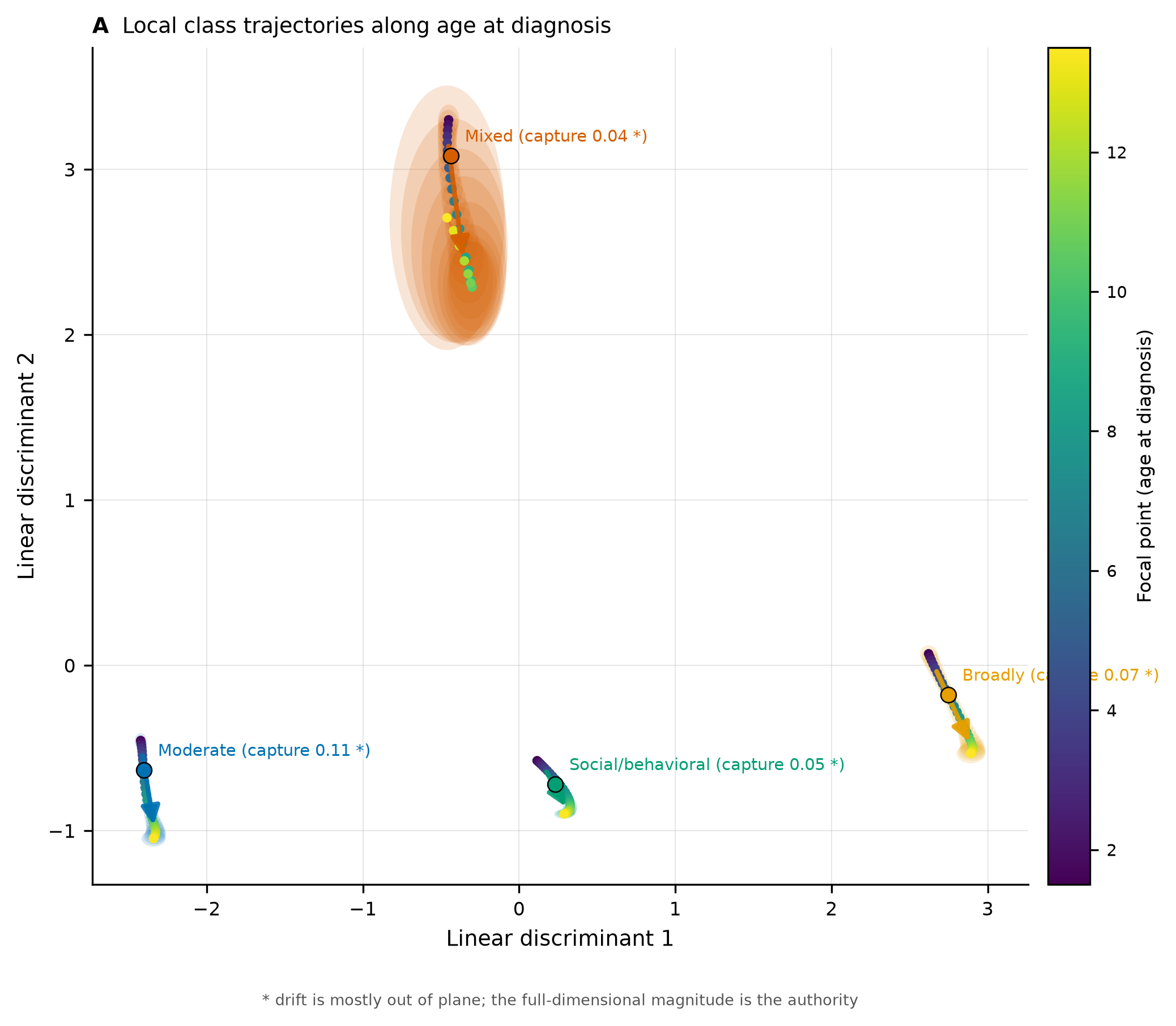
Four class centroids in the discriminant plane, each with a short local trajectory along age at diagnosis — The same trajectories along age at diagnosis, coloured youngest to oldest at diagnosis. The developmental class (Mixed ASD with developmental delay) is the largest mover on this axis, yet its in-plane path is short and its capture fraction is only \(0.04\), so nearly all of that movement leaves the plane. Every class is again flagged (capture below one half), so the drift here is even more out-of-plane than on the era axis and the picture understates it. Rendered by `figures.trajectory_local` (`figures local-trajectory --axis age_at_diagnosis`).#

Corroboration: the score-based test#

A second read asks the same question from the single cached fit, with an analytic null: the score-based invariance test of Merkle and Zeileis [1]. Order the probands by the axis, take the running sum of their class-profile scores, and standardise it into an empirical fluctuation process that converges to a Brownian bridge under the null. It shares no machinery with the effect-size read, so agreement is not circular. At this sample size the test saturates: almost every block rejects at the smallest attainable \(p\)-value and the break confidence sets span nearly the whole axis. Its value is direction and rough location, not magnitude.

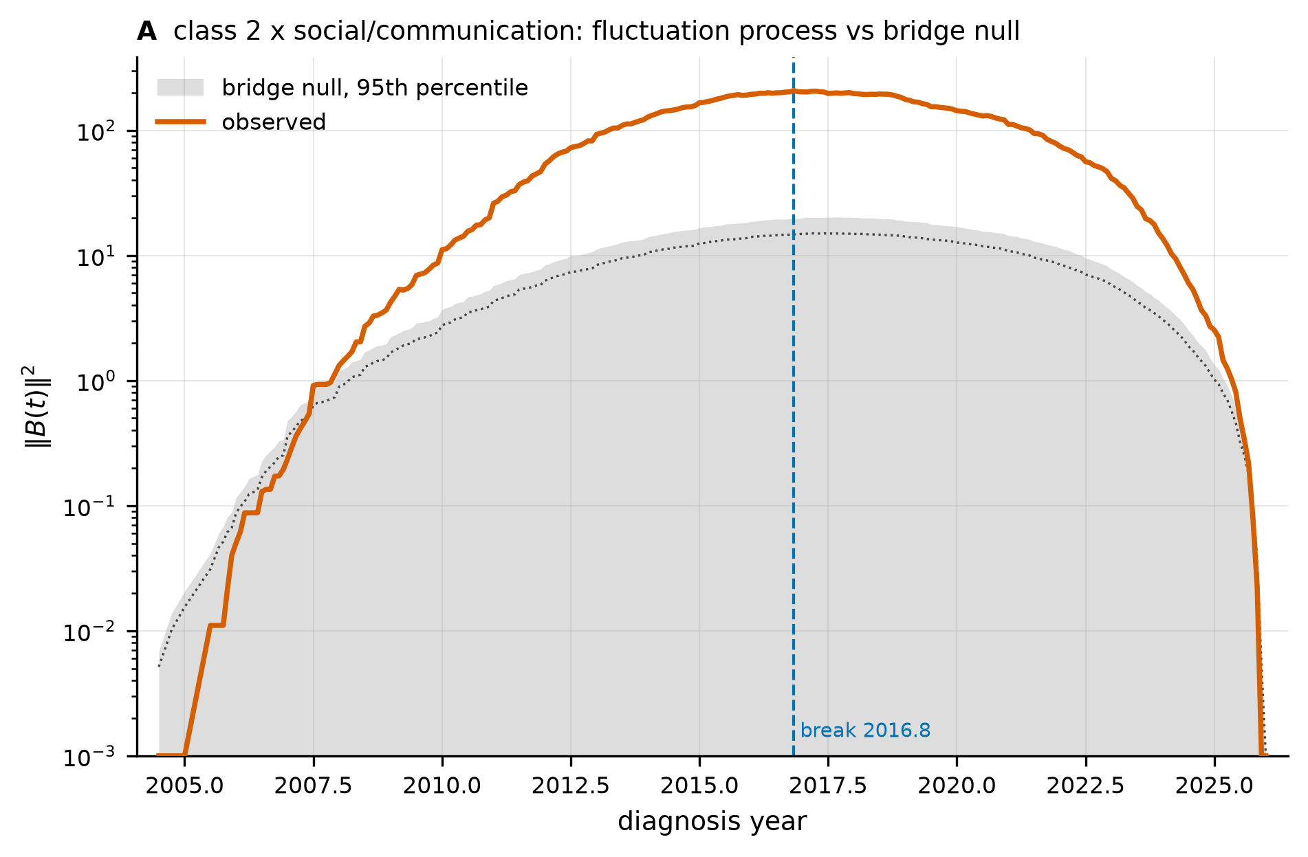
Squared fluctuation process against diagnosis year, an order of magnitude above the simulated bridge null band — The squared fluctuation process of the strongest-drifting block against diagnosis year (note the logarithmic vertical axis), with the simulated bridge null band beneath. How to read it: a stable class would sit inside the band; the observed process instead climbs an order of magnitude above it across the whole axis, the signature of a pervasive drift rather than one sharp break. The excursion grows through the 2010s. Rendered by `figures.invariance` (`figures invariance --axis era`).#

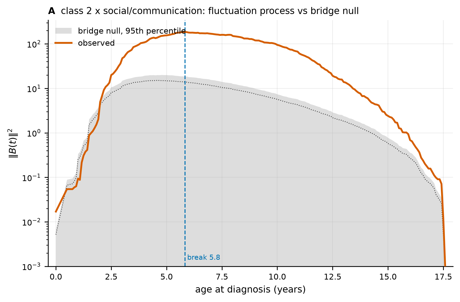
Squared fluctuation process against age at diagnosis, an order of magnitude above the simulated bridge null band — The same read along age at diagnosis, for the strongest-drifting block (the Mixed class on social or communication). The observed process climbs an order of magnitude above the bridge null and stays there across the axis, rising fastest through early childhood and peaking near the estimated break at about six years. As on the era axis, the excursion is broad rather than one sharp step, so the drift is pervasive. Rendered by `figures.invariance` (`figures invariance --axis age_at_diagnosis`).#

The score-based test is the analysis invariance stage.

Handling the null#

For \(H_0^A\) the decision is a per-class magnitude comparison, not a reject-or-not on the bridge \(p\)-value, which saturates: a class’s era or age displacement is above noise if it clears the random ordering, and specific to timing if it also clears the two covariate controls. Along age at diagnosis all four classes clear every control, so \(H_0^A\) is rejected throughout. Along diagnostic era the paired specificity bootstrap rejects at its floor (\(p = 0.0005\)), but per class the rejection is specific only for Moderate challenges and the developmental class; Broadly affected and Social or behavioral drift above noise without clearing their covariate controls, so the era verdict is a rejection that is not uniform across classes.

For \(H_0^D\) the decision is whether the magnitude exceeds the sampling-noise floor and is non-trivial against the separation. It is: the magnitude is distinct from the random floor with its bootstrap band excluding it, and in root-mean-square terms reaches about a fifth of a class gap on era and more on age, so \(H_0^D\) is rejected. The small capture fractions qualify the reading rather than the verdict: the drift is real and sizeable, but mostly outside the plane the figures draw.

Discussion#

The class profiles are not invariant to diagnostic timing. They drift, the drift is larger for age at diagnosis than for diagnostic era, and on era it concentrates in two classes rather than spreading evenly. The movement is high-dimensional, so the discriminant-plane figures understate it, and the full-dimensional separation-scaled magnitude is the authoritative read. The read is conditional on the pooled fit: it freezes the reference responsibilities and reweights, measuring where the class centroids sit along the axis. Whether the drift has a direction, and how the class proportions move, are separate questions taken up in the sibling articles.