Choosing the specificity controls

The question

The specificity check asks whether a class drifts more along diagnosis timing than along an ordering that carries no real structure. The confirmatory control is the random order alone: it is the one baseline guaranteed to be orthogonal to the timing shift without any assumption about what else might be. Any covariate control (household income, area deprivation) instead assumes the covariate is orthogonal to timing, an assumption the data cannot guarantee, so the manuscript reports the random-order control only. This page is retained for transparency: it documents an earlier covariate screen, why the random order is the assumption-free floor, and why the covariate candidates were set aside rather than trusted.

The result

The random order is the assumption-free control: a class is above the noise floor when its endpoint displacement clears it (mean about \(0.09\) separation units, a fraction of the mean inter-class gap). All four classes clear the random floor on both axes. The covariate screen below was an attempt to find harder, timing-orthogonal controls; two graded near-complete covariates survived it (household income and area deprivation), but both require assuming orthogonality to timing, so they are reported here as context rather than as the confirmatory bar. Two roles are excluded on principle whatever their numbers: the 238 clustered features (ordering by one moves the class centroids by construction) and other phenotype measures such as symptom totals or IQ (a non-null ceiling that also tracks timing).

The comparison the check makes

A large displacement on its own does not separate genuine drift from noise accumulated over many features, because the norm of pure sampling noise is positive too. The specificity check reads the same separation-scaled endpoint displacement along control variables and asks whether the timing axes exceed them. A class is above the noise floor if it clears a random ordering, and specific to timing if it also clears a real covariate that is not the mechanism. The mechanics of the endpoint displacement are in invariance as an effect size; this page is about which controls earn a place in the comparison.

Two roles are disqualified before any number

The variables split by role, and two roles cannot be negative controls whatever their numbers say.

The classes are defined in the space of the 238 clustered features, so ordering probands by one of them, and reading how the class centroids shift along that order, is circular: the centroids differ on that feature because the classes were built to. Symptom totals and ability scores that are not in the 238 are the second excluded role. They are still phenotype, correlated with the clustered features by construction, so ordering by them moves the centroids for a real but non-timing reason, a ceiling rather than a null. Cognitive impairment and IQ belong here, which is why neither can serve as a control even though both are proband-level covariates.

This is why a screen that simply ranks every variable by its correlation with timing and picks the lowest would go wrong. The RBS-R total has a rank correlation with year of diagnosis and with age at diagnosis of about \(0.03\) to \(0.04\), cleaner than area deprivation, yet it is a total over clustered instrument items and moving probands along it would shift the centroids by construction. Orthogonality to timing is necessary but not sufficient. A control must also not be the phenotype, and a correlation cannot see role.

Screening the legitimate pool

The legitimate pool is the proband-level covariates that are not the phenotype. Each was screened on the reference cohort (SPARK 2026-03-23, 11,704 probands) for its rank correlation with the two timing axes, whether it is graded enough for the trajectory to have an axis to walk, and its missingness.

Candidate	Role	Distinct values	Missing	\(\lvert\rho\rvert\) era	\(\lvert\rho\rvert\) age
Random ordering	floor	11,704	0%	0.003	0.003
Area deprivation (2019 ADI)	covariate	100	10.6%	0.043	0.035
Household income (9 bands)	covariate	9	1.3%	0.070	0.041
Number of ASD siblings	covariate	6	30.9%	0.021	0.027
Sex	covariate	2	0%	0.113	0.106
Race (white indicator)	covariate	2	0%	0.243	0.175
Family type	covariate	3	0%	0.208 (eta)	0.082 (eta)
RBS-R total	phenotype	128	0%	0.031	0.037
SCQ total	phenotype	40	0%	0.278	0.227
Full-scale IQ	phenotype	101	93.4%	0.173	0.328
Registration year	timing	12	0%	0.692	0.261
Age at evaluation	timing	14	0%	0.249	0.410

The screen validates itself at both ends. The variables that are timing by construction, registration year and age at evaluation, top the correlation ranking as they should, and the random ordering sits at \(0.003\). Between them, only two covariates are graded, close to timing-orthogonal, and nearly complete: household income and the area deprivation index. Sex correlates with both timing axes more than either (about \(0.11\)) and is binary, so its trajectory is degenerate; its earlier low displacement was that degeneracy, not evidence of no phenotype signal. The white-race indicator and family type are more timing-confounded still. The pool of clean graded covariates in SPARK is small, so the panel is short by necessity, not by neglect.

Is household income too high?

Household income is the hardest control: its per-class endpoint displacements reach \(0.29\) for the Broadly affected class and \(0.27\) for the developmental class, and that is what turns two era classes from specific to not specific. So the fair question is whether income is a legitimate strong socioeconomic gradient or is acting like the IQ and cognitive-impairment proxies the previous section excluded. Placing every axis on the same displacement scale answers it.

Axis	Role	Mean endpoint (sep. units)
Random ordering	floor	0.087
Area deprivation	covariate	0.139
Household income	covariate	0.209
SCQ total	phenotype ceiling	0.427
RBS-R total	phenotype ceiling	0.649

Income sits in the middle of the scale, above the random floor and area deprivation but far below the phenotype ceiling that the clustered-instrument totals set at \(0.43\) to \(0.65\). A phenotype proxy would land at that ceiling; income is less than half of it. Its correlations tell the same story: income is uncorrelated with cognitive impairment (Spearman \(|\rho| = 0.02\)), the cleanest severity marker, so it is not a disguised severity axis; it correlates \(0.50\) with area deprivation, confirming it is a socioeconomic measure; and it correlates \(0.31\) with the RBS-R total, a real but modest social gradient in symptom severity. Income reads higher than area deprivation because household income is a cleaner socioeconomic signal than neighbourhood deprivation, not because it is phenotype.

The same read explains why IQ and cognitive impairment cannot stand in as the ceiling here. Both came back near or below the floor (\(0.06\) and \(0.0\)), degenerate because cognitive impairment is binary and IQ is present for only a small, selected minority. Only the graded clustered totals read as a real phenotype ceiling.

So income stays. Its height is the control working, not failing. Dropping a valid control because it is stringent would select controls that flatter the timing result, the bias the screen exists to avoid. The screen chose income on validity grounds, blind to its magnitude, and swapping the earlier sex control (an easily cleared bar at \(0.05\)) for income (a stringent bar at \(0.21\)) makes the specificity test harder, not easier.

The panel

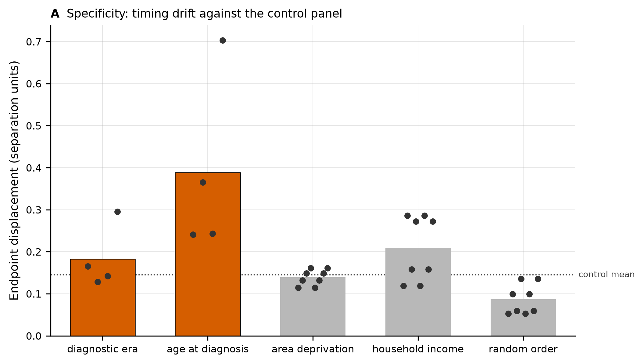
Endpoint displacement by axis, in separation units, on the reference release. The two timing axes (highlighted) carry a dot per class; the control panel is area deprivation, household income, and a random ordering. The dotted line is the control mean.

The panel is a random ordering (the floor, about \(0.09\)), household income (about \(0.21\)), and area deprivation (about \(0.14\)). Read per class rather than on the between-class mean, because a mean hides drift concentrated in one class: a class is above the noise floor if its endpoint clears the random ordering, and specific to timing if it also clears the household-income and area-deprivation controls. Along age at diagnosis all four classes clear every control. Along diagnostic era the Moderate challenges and developmental classes clear the covariate controls while the Broadly affected and Social or behavioral classes clear only the random floor, so their era drift is above noise but no larger than a real socioeconomic gradient in the same classes. This is the same two-class era verdict the earlier sex-and-deprivation panel gave, now standing against the stronger bar.

Limits

The controls are read on the same frozen reference and the same endpoint displacement as the timing axes, so they inherit its assumptions: the comparison is where the class centroids sit along an ordering, not a re-estimated partition. SPARK’s supply of graded, non-phenotype, timing-orthogonal covariates is thin, so the panel rests on two socioeconomic measures that correlate with each other at \(0.5\); they are not independent readings of the same idea so much as one construct measured at the household and the neighbourhood. The screen’s correlations and the ceiling placement are a design-time read on the reference cohort, quoted here as the evidence for the panel rather than as a pipeline stage. What the page settles is narrow and firm: the negative controls are chosen by role and by a timing-orthogonality screen, not by convenience, and the one control that decides the era verdict is a genuine socioeconomic gradient, not leaked phenotype.