Replicating in the SSC#
The question
Do the four classes reappear in a second, independent cohort? The reproduction and the stability checks are all within SPARK. This check fits a fresh model on the SPARK features shared with the SSC, projects it onto the SSC, and asks whether the seven-category class profiles agree across the two cohorts, the measure the authors used to declare replication.
The result
The classes replicate. The SPARK model projects onto \(798\) SSC probands across the \(106\) shared features, and the seven-category profiles correlate at \(r = 0.90\), beyond a permutation null (\(p = 0.006\)). A proband bootstrap puts a \(95\) per cent interval of \([0.79, 0.94]\) on that value, which spans the authors’ published \(r = 0.927\). Every per-category correlation sits at \(0.85\) or above, and their bootstrap intervals are wide: six of the seven cover the value Litman et al. (2025) report, developmental among them. The interval stays wide because the SSC sample is small and its two smallest classes hold about \(4\) and \(5\) per cent of it.
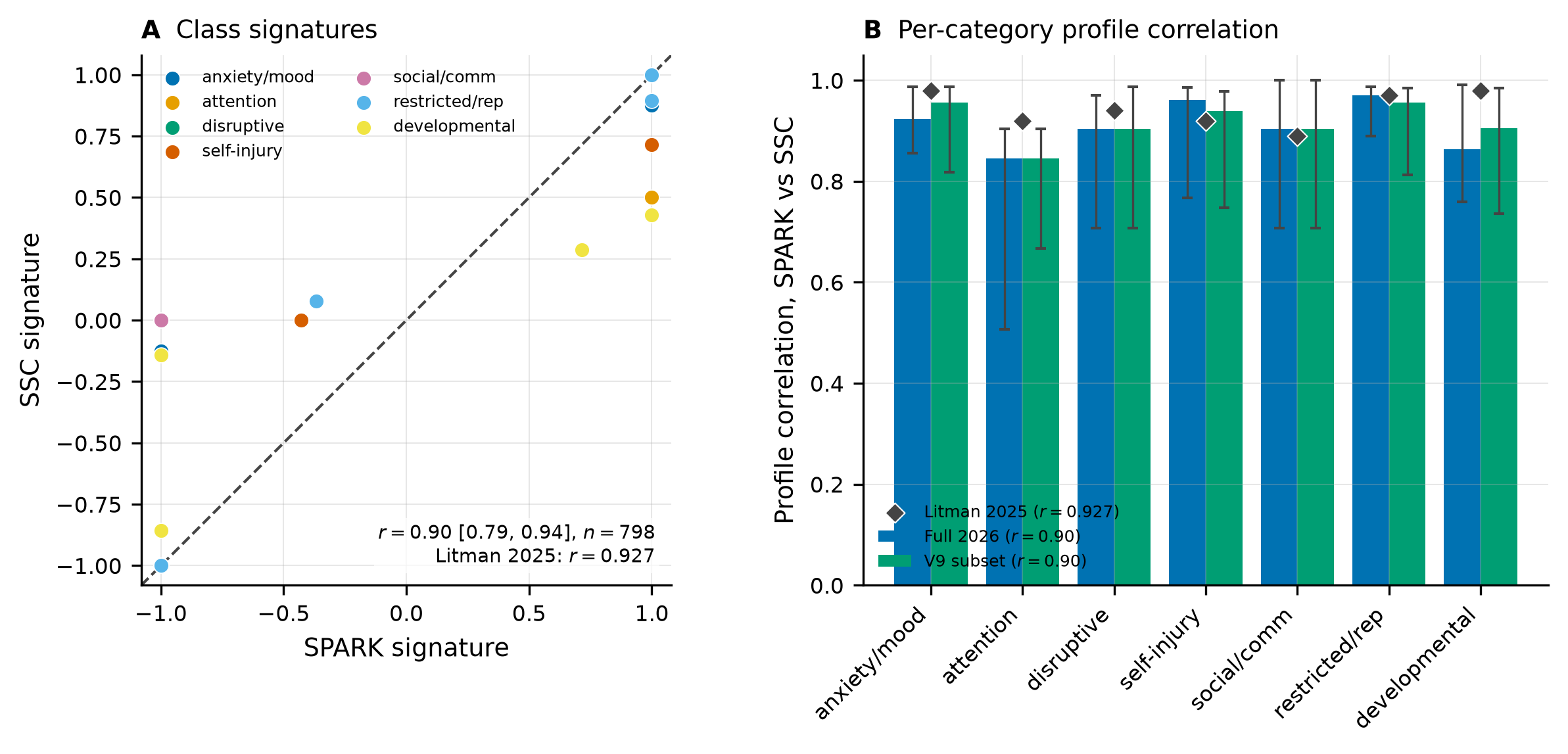
Cross-cohort replication, from analysis replicate runs projecting the SPARK model onto \(798\)
SSC probands. (A) Every class-by-category signature value, SSC against SPARK, around the line of
equality (\(r = 0.90\), \([0.79, 0.94]\)), with the authors’ overall \(r = 0.927\) alongside. (B) The
per-category correlation for two training conditions, the full 2026-03-23 release and the
cohort cut back to the records present at the authors’ V9 freeze (see
subsetting the cohort to the V9 freeze), against
the values Litman et al. (2025) report (diamonds). Whiskers are the proband-bootstrap \(95\) per
cent interval on each per-category correlation. The two conditions track each other (overall
\(r = 0.90\) for both), so the SPARK records the model trains on do not drive the replication;
developmental reads \(0.86\) on the full release and \(0.91\) on the subset, against the published
\(0.98\), its wide interval covering that value.#
The overall correlation#
On the SSC \(15.3\) release the SPARK model projects onto \(798\) probands, across the \(106\) features the two cohorts share, and the seven-category profiles correlate at \(r = 0.90\). The permutation null places that value beyond chance: of the \(172\) label shuffles that yield a defined correlation, none reaches the observed \(r\), so the calibrated \(p\)-value is \((1 + 0) / (1 + 172) = 0.006\). A shuffle that flattens a class profile gives an undefined correlation and drops from the null, so the bound would tighten with more permutations, but it already places the observed correlation outside the null.
Resampling the \(798\) probands \(500\) times, the labels held fixed, puts a \(95\) per cent interval of \([0.79, 0.94]\) on the overall \(r\). That interval is wider than the reproduction’s \([0.89, 0.92]\), because the SSC sample is small and its two smallest classes hold about \(4\) and \(5\) per cent of it, but it spans the authors’ published \(r = 0.927\). The replication is therefore above the permutation null and consistent with the published value, if less precise than the within-SPARK reproduction.
The per-category correlations#
Each category’s correlation is taken over the four classes alone, the coarsest of the seven readings, so it moves sharply when one class shifts. The bootstrap makes that imprecision explicit: the per-category intervals are the whiskers in panel B, and they are wide. The point estimate, its interval, and the published coefficient for each category:
Category |
This work |
\(95\) per cent interval |
Litman 2025 |
|---|---|---|---|
restricted or repetitive |
\(0.97\) |
\([0.89, 0.99]\) |
\(0.97\) |
self-injury |
\(0.96\) |
\([0.77, 0.99]\) |
\(0.92\) |
anxiety or mood |
\(0.92\) |
\([0.86, 0.99]\) |
\(0.98\) |
disruptive behaviour |
\(0.90\) |
\([0.71, 0.97]\) |
\(0.94\) |
social or communication |
\(0.90\) |
\([0.71, 1.00]\) |
\(0.89\) |
developmental |
\(0.86\) |
\([0.76, 0.99]\) |
\(0.98\) |
attention |
\(0.85\) |
\([0.51, 0.90]\) |
\(0.92\) |
Six of the seven intervals cover the published coefficient; only attention’s, at \([0.51, 0.90]\), sits just below the published \(0.92\). Developmental has the largest gap in point estimates, \(0.86\) against \(0.98\), but its interval reaches \(0.99\), so the gap is within the sampling noise of a four-class correlation on a small cohort. The overall \(r\), over the full four-class, seven-category profile, is the stabler summary; the per-category values are read with their intervals rather than as point estimates.
Developmental is worth a note beyond its width. It is the one category the SSC assembles entirely
from parsed background-history milestone ages: of its eleven features the SSC supplies the nine
milestone ages, while the second-phrase milestone (combined_phrases_age_mos) and the school
item (repeat_grade) have no SSC source, so it carries none of the standard-instrument items the
other categories draw on (see
parsing the SSC milestone ages). Its point estimate also
rests on the two smallest projected classes, about \(4\) and \(5\) per cent of the SSC, so it is
estimated from few probands. Both properties widen the interval rather than shift the centre.
The training cohort is not the cause#
Retraining on the cohort cut back to the records present at the authors’ V9 freeze (the second condition in panel B; see subsetting the cohort to the V9 freeze) gives an overall correlation of \(r = 0.90\), matching the full release, with developmental at \(0.91\) against \(0.86\) on the full release. Developmental is no lower on the smaller, earlier cohort, so whatever separates it from the published value sits on the SSC side of the projection, in the milestone ages and the thin projected classes, not in the SPARK training records.
Class sizes under projection#
The class sizes under projection are more skewed than under the SPARK fit. The SSC places about \(62\) per cent of its probands in the largest class, against \(39\) per cent under the shared-feature SPARK fit, and only about \(4\) and \(5\) per cent in the two smallest, against \(8\) and \(16\) per cent in SPARK. The replicate stage fits one model on the shared features and carries the class ids straight across both cohorts, so these are class sizes under a single model, not a re-alignment to the named reference.
How the projection works#
Fitting on the shared features and projecting
The replicate stage fits a fresh model on SPARK restricted to the features shared with the SSC,
then that fitted model predicts class labels on the SSC. Because both cohorts pass through the one
model, the class ids already correspond, so no cross-cohort label alignment is needed. The
replication measure is the correlation of the seven-category profiles between the two cohorts, the
currency the authors used to declare replication.
Two points of care. StepMix validates a prediction input by its feature count, not its column names, so the SSC measurement matrix is reindexed to the exact SPARK column order before prediction. And the released code reports the correlation without a null; the package adds a permutation null that shuffles the SSC class labels and recomputes the correlation, so the observed value is read against chance.
Caveats#
Two caveats qualify the replication. The SSC milestone ages are parsed from free text here, not read from the authors’ unreleased hand-cleaned file, and that parse is the whole of the developmental category, the category with the widest interval. And the shared-feature complete-case reduction leaves \(798\) probands, below the full SSC release, so the replication is read against the published value rather than offered as an exact reproduction.