The score-based invariance test#
The corroborating machinery for the invariance read of H_0^A and H_0^D: are the class profiles invariant, and is any drift small? (\(H_0^A\)). The drift stages ask whether the class profiles are invariant along an axis by refitting the mixture inside strata; the analysis invariance stage asks the same question from the single cached fit instead, with an analytic null and no refitting, following the empirical fluctuation process of Merkle and Zeileis [1]. It shares no machinery with the effect-size read, so agreement between the two is not circular. This guide sets out the casewise score, the fluctuation process and its bridge null, the two statistics, the focal blocks, and the correctness gates; the hypothesis article carries the verdict and the reading.
The casewise score#
At the maximum-likelihood estimate, each proband contributes a score to every class-profile
parameter, the gradient of its log-likelihood with respect to that parameter. For a mixture,
Fisher’s identity makes this the responsibility times the emission gradient: the casewise score
of proband \(i\) on the class-\(k\) value of feature \(j\) is \(r_{ik}\,\partial_\theta \log
f_j(x_{ij};\theta_{jk})\), where \(r_{ik}\) is the posterior responsibility (the model’s
predict_proba).
The focal parameters are the class-conditional locations, the profiles the whole analysis measures. Each emission type has an exact score:
a Gaussian mean gives \(r_{ik}(x_{ij}-\mu_{jk})/\sigma^2_{jk}\);
a Bernoulli probability gives \(r_{ik}(x_{ij}-p_{jk})/(p_{jk}(1-p_{jk}))\);
a categorical outcome \(l\) gives the multinomial-logit score \(r_{ik}(\mathbb{1}[x_{ij}=l]- p_{jkl})\).
On the reference release the measurement features are 38 continuous, 33 binary and 167 categorical, so the categorical block is the majority and is scored rather than dropped. The outcomes of a categorical feature sum to a redundant direction, because the outcome probabilities are a simplex; the whitening below removes it, so no reference outcome is chosen by hand.
The fluctuation process and its bridge null#
Order the probands by the axis and take the running sum of their scores. Standardise it by the inverse square root of the outer-product-of-gradients covariance of the focal block, which decorrelates the block’s dimensions, and scale by the root of the sample size. The result is the empirical fluctuation process \(B(t)\), \(t \in [0, 1]\). Because the fit forces the full-sample score to zero, the process is pinned to zero at both ends; a small residual tilt, from an optimiser that stops at a tolerance or from an axis that covers most but not all probands, is removed by a linear tie-down. Under stability \(B(t)\) converges to a Brownian bridge.
Two functionals read the process:
The maxLM is the largest excursion, powerful against an abrupt break, and its location is the estimated break. The Cramer-von Mises is the integral, powerful against a gradual drift. The null is drawn by simulating many independent \(d\)-dimensional Brownian bridges on the axis’s own time grid (\(d\) the effective block dimension) and reading the same functional off each. This is a Gaussian-process simulation of microseconds, not a model refit, so the \(p\)-value is analytic. The estimated break carries a confidence set, the axis positions whose excursion clears the null’s maxLM critical value.
A signed directional slope, the ordinary-least-squares slope of each focal parameter’s score on the axis, reports the sense of a drift: a systematic trend rather than a fluctuation about zero.
Focal blocks and multiplicity#
The process is read per block. A whole-class block pools every location parameter of a class; a class-by-category block restricts a class to one feature category, so a drift can be localised to a class and a symptom domain. Significance is Benjamini-Hochberg controlled across the blocks within an axis, the repo convention for the strata-by-class tests. The whole-class blocks have a much larger dimension than the category blocks, so their raw maxLM is larger; the two are compared by \(p\)-value, not by raw statistic.
The correctness gates#
The test is a \(p\)-value engine, so its scores are validated before any real reading is trusted. Three gates, on synthetic data, guard it:
the analytic casewise score matches a central finite difference of the per-sample log-likelihood to machine precision, for every emission type;
a synthetic mixture with a planted mean drift along the axis yields a small \(p\) in the drifted block and localises the break near the planted point;
with no drift the \(p\)-values are uniform, so the analytic null is calibrated rather than assumed.
The score validation is the load-bearing one: a wrong gradient would invalidate every \(p\)-value, so the same finite-difference check is also run on the real reference fit before it is read.
Running it#
uv run analysis invariance --axis age_at_diagnosis
uv run analysis invariance --axis era
The stage resolves the measurement-only reference (the analysis fit --no-covariates fit), joins
the axis to its probands, drops any with a missing axis value and reports the coverage, and writes
one row per block with the two statistics, their bridge \(p\)-values, the Benjamini-Hochberg
decisions, the estimated break and its confidence set, and the directional slope. It also stores
the fluctuation process of the strongest-drifting category block, which uv run figures invariance --axis age_at_diagnosis draws against the simulated null band.
--n-simulations sets the number of null bridges (2000 by default), --seed the null draw, and
--max-grid the largest evaluation grid (tied axis values are collapsed, then thinned to this).
The run hash folds in the reference fit, the axis, the focal-block specification, the number of
simulations and the seed, so each configuration caches as its own run.
The fluctuation process#
The figure draws the squared norm \(\lVert B(t) \rVert^2\) of the strongest-drifting category block against the axis, with the pointwise envelope of the simulated bridge null shaded beneath (note the logarithmic vertical axis). Both curves are arches, pinned to zero at each end: the cumulative score starts at zero over no probands and returns to zero over all of them, because the full-sample score vanishes at the fit. The null band traces the bridge variance \(t(1-t)\), widest in the middle where a process tied at both ends has the most room to wander. A class that were stable would sit inside that band; the observed curve instead climbs an order of magnitude above it across the whole axis, the signature of a pervasive drift rather than a single sharp break.
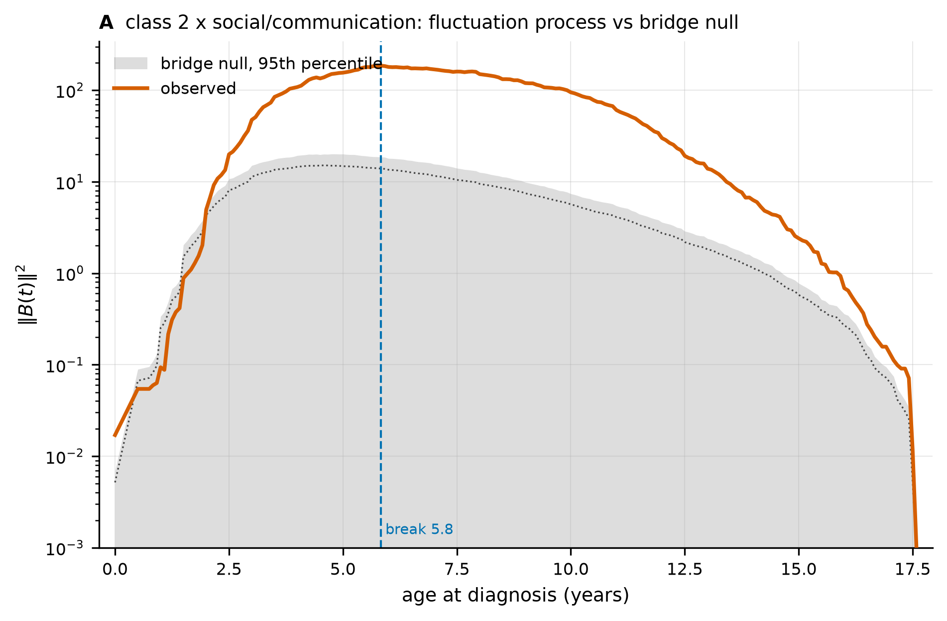
Age at diagnosis, the strongest class-by-category block (Social or behavioral, social and communication features). The observed process (orange) sits well above the bridge null band (grey) from early childhood on, and peaks near the median age at diagnosis. The peak is labelled a break, but its breadth and wide confidence set mark it as a diffuse, continuous drift; the peak of a smoothly drifting process falls at the axis median by construction, not at a change point.#
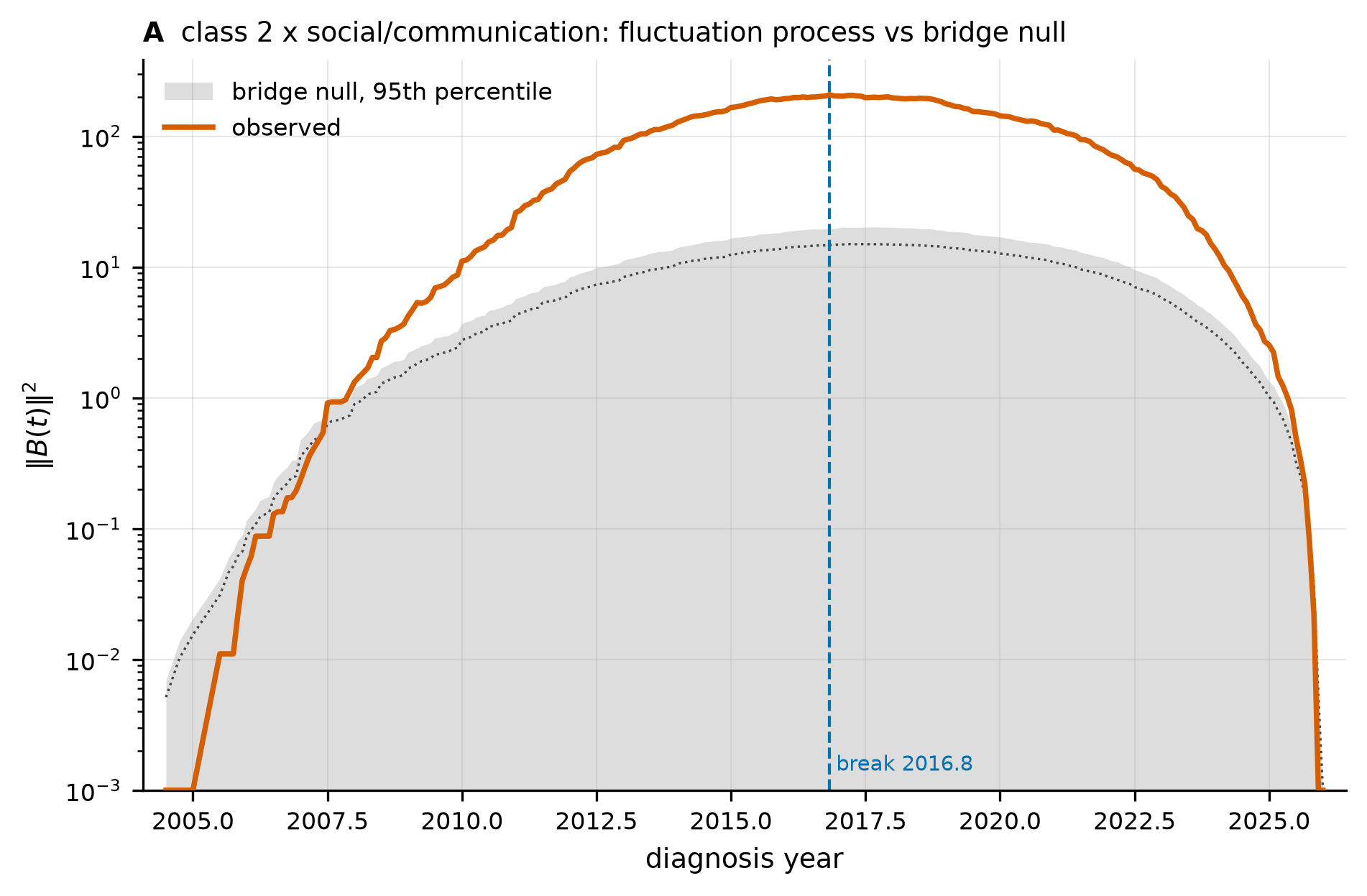
Diagnostic era, the same block. The excursion above the null band grows through the 2010s, with the social and communication scores trending upward with diagnosis year (a positive directional slope). The break near 2016 is again close to the median diagnosis year, so it reads as the centre of a continuous change over the era rather than an abrupt one.#