Attributing a class’s movement

The drift step reports how far a class moved as one number per class. That number says a class changed; it does not say what changed or for whom. This stage opens the number up, along two lines: which features carry the shift, and which probands changed class between the two fits. A movement then reads as “these features, these people” rather than a single distance.

Both readings are cheap consumers of the stored fits. The reference fit and the stratum fits are already on disk, so attribution re-reads them and does no re-fitting. Because its inputs are two labellings on a shared proband index (plus the fit summaries and their alignment), it is indifferent to how the second labelling was produced: a hard stratum bin, a kernel-weighted focal point, or a partition-tree node all present the same way, so the same attribution runs on any of them.

What moved: decomposing the centroid shift

The drift distance is a single number built from the per-feature centroid shift. It can be split back into per-feature contributions that sum to it, so the movement gains a ranked feature breakdown that adds up to the distance the drift stage reported.

The Mahalanobis split is the default, and it matches the default drift distance. The squared Mahalanobis distance is the quadratic form \(\Delta\mu^\top P \Delta\mu\) in the centroid shift \(\Delta\mu\) and the shrunk within-class precision \(P\). That form expands term by term into per-feature contributions \(c_i = \Delta\mu_i (P\Delta\mu)_i\) that sum to the squared distance, so a coordinated shift across a correlated block of symptoms is charged to the block once. A contribution can be negative, when a feature’s shift offsets a correlated block, which the diagonal split cannot show.

The standardised split is the covariance-blind cross-check: \(c_i = (\Delta\mu_i / \sigma_i)^2\) in pooled-standard-deviation units, non-negative, summing to the total squared standardised shift. A feature that ranks high here but low under the Mahalanobis split is one whose apparent movement is shared with a correlated block rather than its own.

Each per-feature contribution is reported with its signed shift (the direction the class moved on that feature) and its literature category, and the contributions are also summed into the seven categories, so the movement reads at the level of the categories as well as the individual features. Every feature is kept in the category totals, blanks and unlisted features under unmapped, so the category totals sum to the same distance the per-feature contributions do.

Who moved: movers against stayers

The second reading is at the level of the probands. A stratum is a subset of the pooled cohort, so every proband in it carries both labellings: the reference class and the stratum-fit class. A class can move in two ways, and both count. It can shed members (leavers, reference members the stratum fit drops) and it can absorb members (joiners, stratum-fit members the reference did not assign there). A class that keeps every member but pulls in new ones has still drifted, so a leaver-only view understates it; the churn (leavers and joiners against the stayers, one minus the Jaccard overlap) is the honest count. Contrasting the churned probands with the stable core says what marks the probands whose membership changed.

The contrast is a swappable method over a feature frame, so the same movers and stayers can be read by more than one model:

• The univariate contrast is the default: a standardised mean difference (Cohen’s \(d\)) per feature between movers and stayers, positive when the movers score higher, with a Welch test and Benjamini-Hochberg control across features. It is model-free, fast, and always defined, the first read on what marks the movers feature by feature.

• The logistic contrast fits an L1-penalised logistic regression of mover status on the standardised features, so its signed coefficients rank the features that jointly distinguish movers from stayers and correlated features share the credit rather than each scoring the marginal difference.

The contrast runs over a feature frame, which is the one lever that decides what the movement is explained by. It is the clustered features for now; the held-out SPARK variables (cognitive level, area deprivation, the measurement-to-diagnosis lag) and, later, the genetic scores are the same interface, so the question “what marks the probands who moved” extends to them without new attribution code. That extension is where the confound-versus-signal reading begins: a movement explained by cognitive level is read differently from one that is not.

The outputs

The stage writes four tables per axis: the per-feature decomposition (contribution, signed shift, and category for every feature and class), the per-category totals, the churn contrast (the ranked feature attributions), and a per-class headline (the stayer, leaver, and joiner counts, the churn and the alignment overlap, and the leading feature on each of the two readings). The headline is the “what and who moved” table; the other three carry the detail behind it.

The figures package draws two figures from these tables. The first sets each class’s churn across the strata beside the categories that carry its shift.

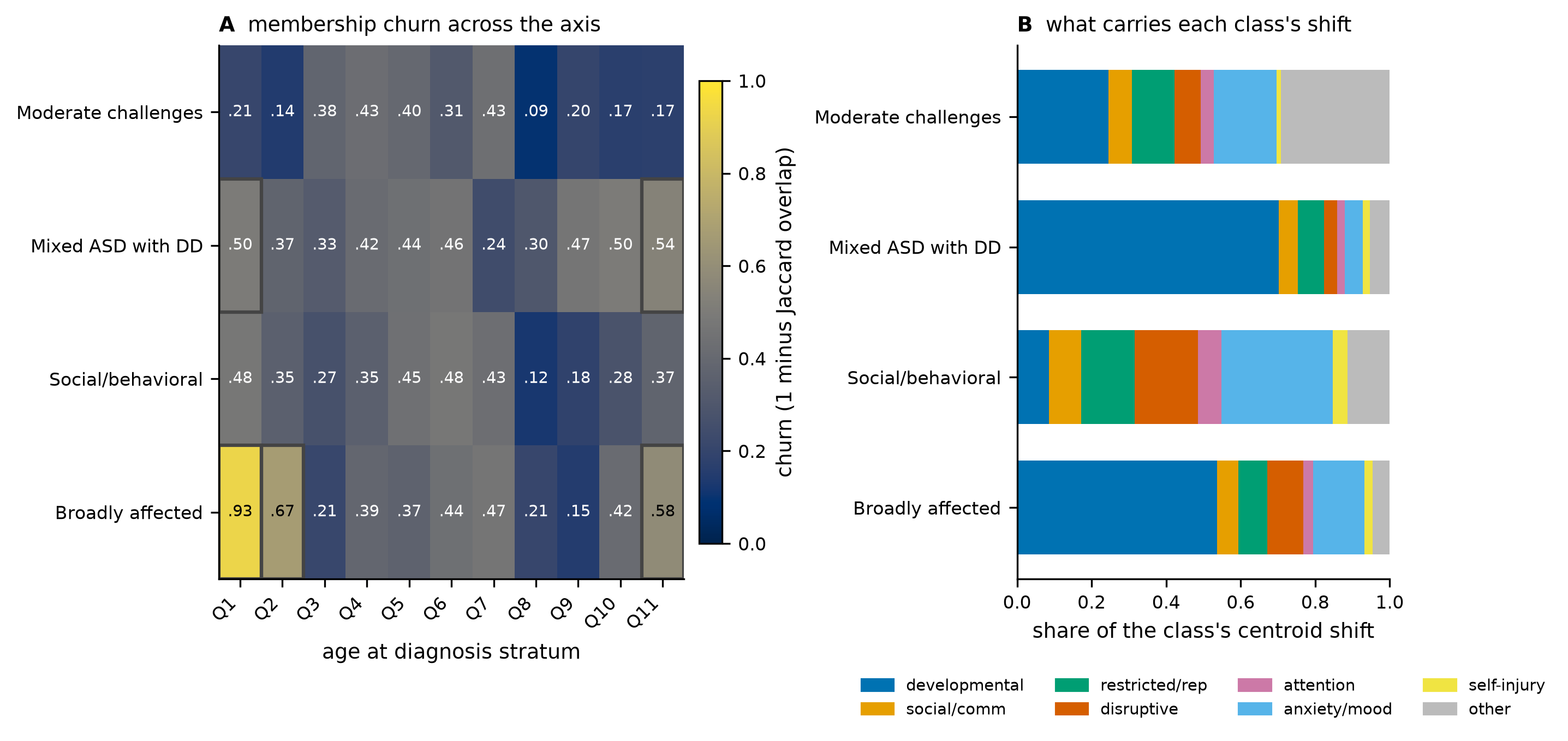
Each class’s membership churn across the age-at-diagnosis strata (panel A), with a box on the reorganised cells, beside the category composition of each class’s centroid shift (panel B).

The reorganised cells (a box in the left panel, where the Jaccard overlap is below one half) are where the membership scattered rather than the centre shifting. The second figure takes each class at the stratum where it churns most and shows the features that most separate the probands that changed class from the stable core.

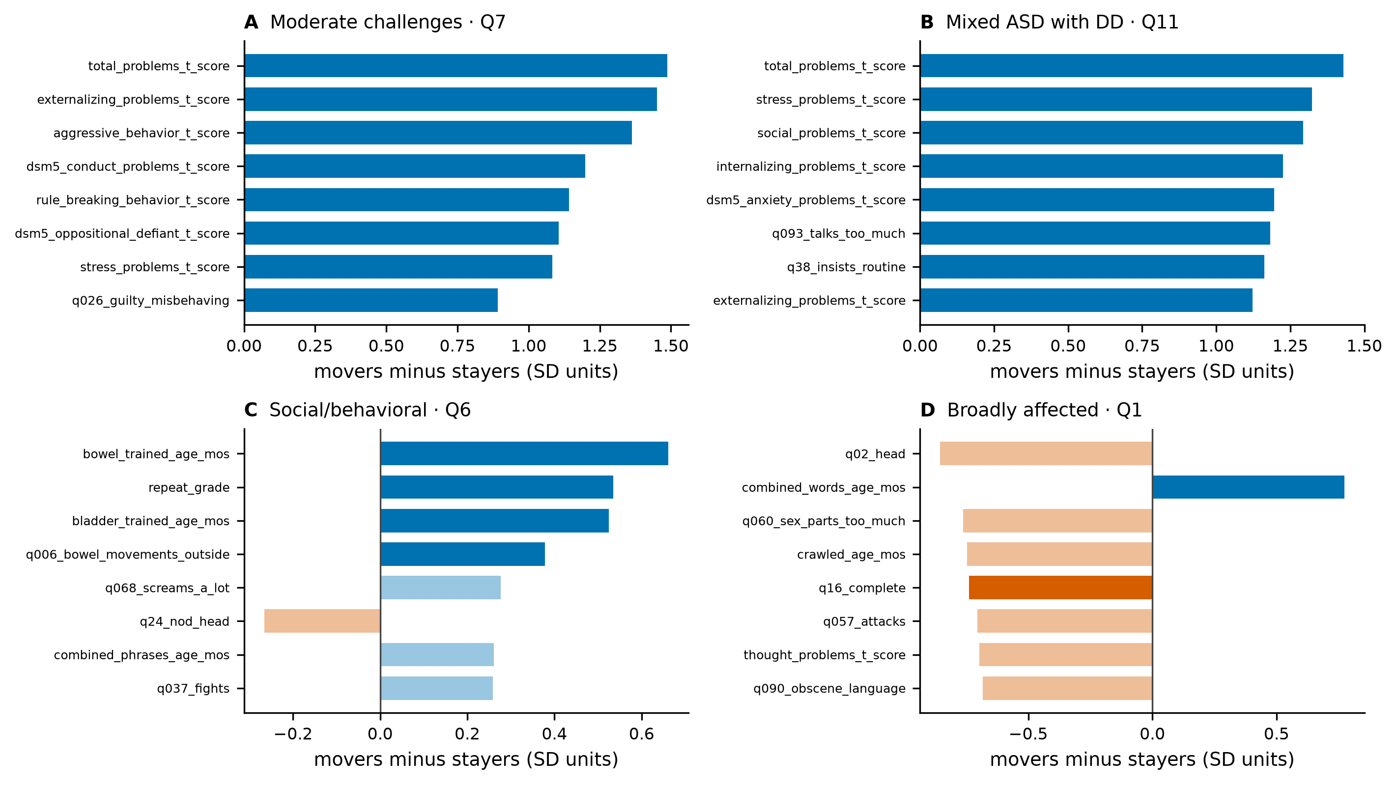
For each class, at its peak-churn stratum, the features that most separate the probands that changed class from the stayers, as a signed standardised mean difference.

The decomposition and the contrast are descriptive readouts of an already-measured drift, not a new test, so they sit outside the pre-registered confirmatory freeze. They interpret a movement; they do not decide whether it is real.

Running the stage

uv run analysis attribute --axis age_at_diagnosis --decomposition mahalanobis --contrast univariate

--decomposition takes mahalanobis (the default) or standardised; --contrast takes univariate (the default) or logistic; --alignment matches the drift stage’s membership or centroid. The choices enter the run hash, so each caches as its own run. The stage reads the cached reference fit and stratum fits and never re-fits, so trying another decomposition or contrast is a matter of seconds.

The two figures above are built from the run and published into the documentation with:

uv run figures attribute --axis age_at_diagnosis
uv run figures attribute-contrast --axis age_at_diagnosis
uv run figures publish attribution-age
uv run figures publish movers-age