Do demographics explain the drift?#
The question
The class profiles drift along diagnostic era and, more strongly, along age at diagnosis. A natural worry is that the drift is not a change in the phenotype at all but a change in who is in the sample: if later-diagnosed children are richer, or more often boys, or from different family structures, the profile that moves might be tracking that composition rather than autism. This page sets the demographic covariates against the drift and asks whether any of them account for it.
The result
No demographic covariate accounts for the drift. Every covariate’s linear span of the timing axis (its axis \(R^2\)) is near zero, so none has room to explain a time-ordered movement, and the shrinkage is near zero to match. Sex is the only mild mover (up to \(0.07\) of a class’s drift on either axis), consistent with the sex-linked, timing-driven prevalence signal seen in the prevalence drift. The drift is carried by the phenotype (the SCQ and developmental features of the category decomposition and the referent split), not by demographic composition.
The two reads and what they measure#
The conditioning guide sets out the machinery; this page reads the numbers. Two reads run on the cached measurement-only reference, on both timing axes, with no refit. The correlated read orders the cohort by each ordered demographic and asks whether the partition drifts along it, and it is reported in the displacement atlas. The explains read residualises the 238 clustered features on each demographic and asks whether the timing drift shrinks. This screen is descriptive: it carries no new pre-registered null, and the confirmatory hypotheses are unchanged.
The figure#
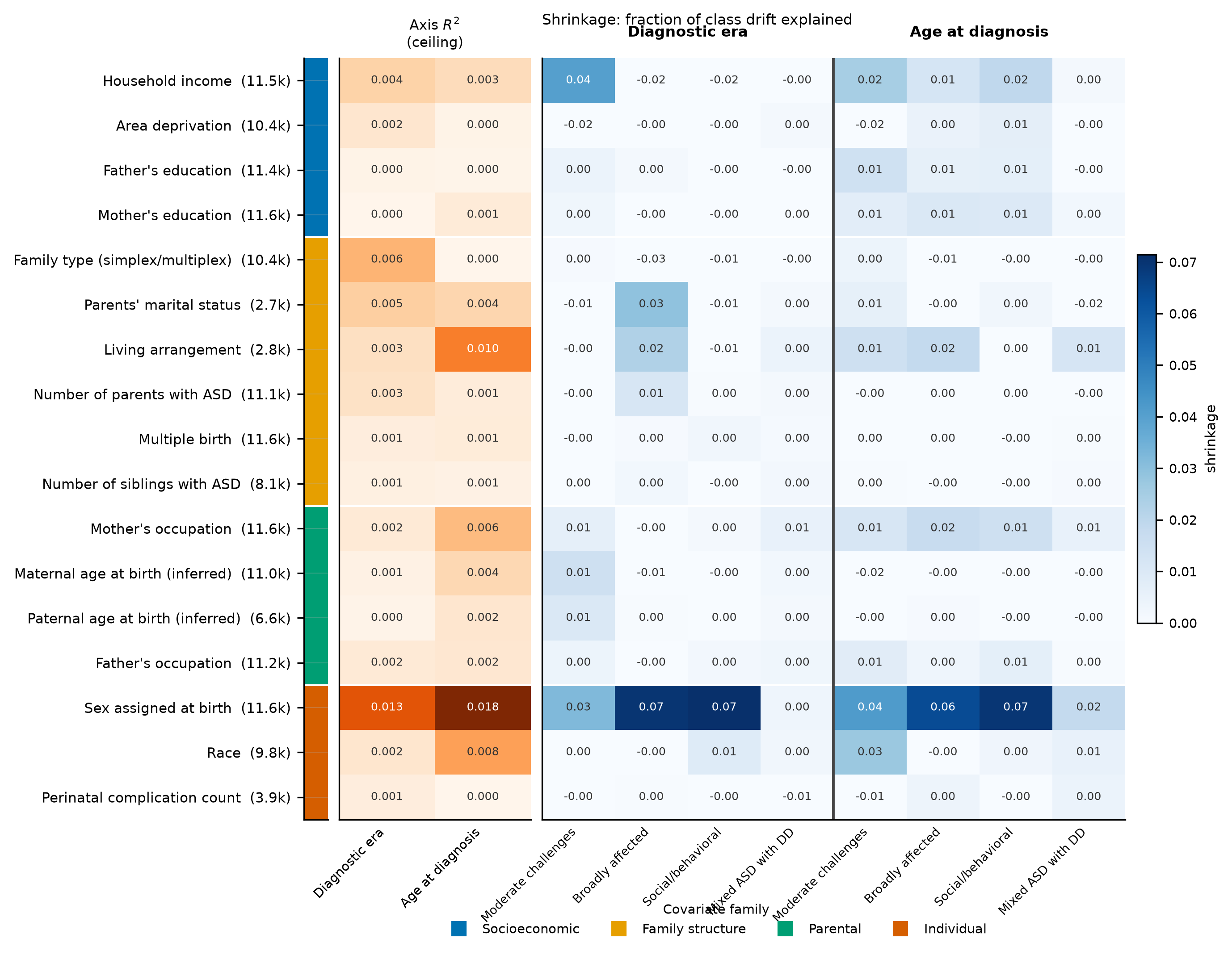
Per-covariate conditioning of the class drift. The orange panel is each covariate’s axis \(R^2\), the fraction of the timing axis it linearly spans (the ceiling on its shrinkage). The blue panel is the shrinkage, the fraction of each class’s drift removed by residualising the phenotype on the covariate, for the four classes on each of the two axes. Rows are grouped by covariate family and annotated with the joined sample size. The axis \(R^2\) column is near zero for every covariate except sex, and the shrinkage panel is near zero to match.#
Reading it#
Read the two panels together, left to right. A covariate can only shrink a timing-ordered drift if it first tracks the timing axis, so the orange axis \(R^2\) column is the ceiling on the blue shrinkage panel. For household income and area deprivation the ceiling is by design: both were chosen as specificity controls precisely because they are near orthogonal to timing, so their near-zero shrinkage confirms the screen rather than surprising it. For the rest, the near-zero ceiling is a fact about SPARK: parental education, family structure, the inferred parental ages, and the perinatal-complication count are nearly flat across diagnosis era and age, so they cannot carry a movement ordered by those axes.
Sex is the exception, and a mild one. It has the largest axis \(R^2\) (about \(0.013\) along era and \(0.018\) along age) and the largest shrinkage (up to \(0.07\) of a class’s drift), concentrated in the same classes whose prevalence shifts with timing. This is the demographic trace of the prevalence drift, not a competing explanation for the profile drift: a small part of the profile movement runs along the same sex gradient that shifts the class sizes, and the rest does not.
Coverage and its limits#
Coverage is a modelling-cohort property, annotated on each row. The registration-complete covariates (sex, income, occupation, education, the parental ages, the family-history counts) join more than ten thousand probands and carry the reading. The survey-version covariates (marital status, living arrangement) survive the coverage floor but join only a few thousand, so their cells are noisier and are read as suggestive rather than settled. Two covariates drop on the cohort for want of variance (the split-biological-family and excluded-family-member flags are near constant among probands), and race enters as a six-way one-hot block rather than an ordering. None of this changes the reading: the well-covered covariates and the thin ones agree that the drift is not a demographic story.